Gradient Descent Code

All the code is written in matlab. Please visits here for a complete version of my code. The neural network code base is in reference to Dr. Chunming Wang's MATH467 project code.

Fixed Gradient Descent Implementation

function fixed_GD()
    function[mse] = meanSquaredError(y, y_pred)
        diff = (y - y_pred).^2;
        mse = mean(diff, "all");
    end

nTrials = 500;
fixed_step_size = 0.01;
epsilon = 1e-3; % minmal convergence error
[xData,yData]=getData(100,2,2338580531);
[network]=createNetwork(2,[3,3,1]);
[Weight]=getNNWeight(network);
Weight=randn(size(Weight));
RMS=NaN(nTrials,1);
[network]=setNNWeight(network,Weight);
prev_yVal = 1;
convergence = -1;
runOnce = 1;
for iTrial=1:nTrials
    [yVal,yintVal]=networkFProp(xData,network);
    [yGrad,~]=networkBProp(network,yintVal);
    f = NaN(1,25);
    for i=1:size(Weight,1)
        f(i) = -2 .* dot(squeeze(yData-yVal), squeeze(yGrad(:, i, :)));
    end
    Weight = Weight - fixed_step_size .* f;
    [network]=setNNWeight(network, Weight);
    RMS(iTrial)=meanSquaredError(yData, yVal);
    if (all(abs(yVal - prev_yVal) < epsilon) && runOnce == 1)
        convergence = iTrial;
        runOnce = 0;
    end
    prev_yVal = yVal;
end
disp(['it converges in ' num2str(convergence) ' iterations.']);
figure;
plot(RMS);
min(RMS)
return
end

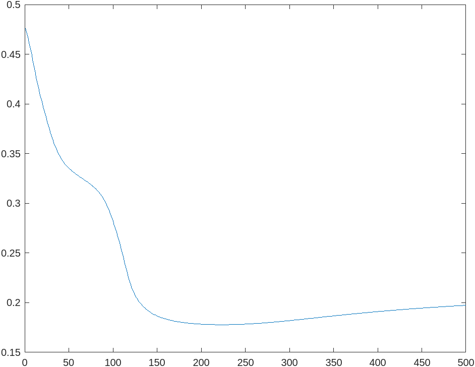
Result

it converges in 306 iterations.

ans =

    0.1778

Analysis

In the code, I use a fixed step size of $0.01$, epoch of $500$, batch size of $100$, convergence error of $10^{-3}$, and a neural network of structure $2\times 3\times 3\times 1$.

Turns out that it takes 306 iterations to converge to a root mean squared error of approximately 0.1778.

Steepest Gradiant Descent

function steepest_GD()
    function[mse] = meanSquaredError(y, y_pred)
        diff = (y - y_pred).^2;
        mse = mean(diff, "all");
    end

nTrials = 100;
steepest_step_size = 1; % start point for minimizing
epsilon = 1e-5; % minmal convergence error
[xData,yData]=getData(100,2,2338580531);
[network]=createNetwork(2,[3,3,1]);
[Weight]=getNNWeight(network);
Weight=randn(size(Weight));
RMS=NaN(nTrials,1);
[network]=setNNWeight(network,Weight);
prev_yVal = 1;
convergence = -1;
runOnce = 1;
for iTrial=1:nTrials
    [yVal,yintVal]=networkFProp(xData,network);
    [yGrad,~]=networkBProp(network,yintVal);
    f = NaN(1,25);
    for i=1:size(Weight,1)
        f(i) = -2 .* dot(squeeze(yData-yVal), squeeze(yGrad(:, i, :)));
    end
    fun = @(a) meanSquaredError(yData, networkFProp(xData, setNNWeight(network, Weight - a .* f)));
    steepest_step_size = fminsearch(fun, steepest_step_size);
    Weight = Weight - steepest_step_size .* f;
    [network]=setNNWeight(network, Weight);
    RMS(iTrial)=meanSquaredError(yData, yVal);
    if (all(abs(yVal - prev_yVal) < epsilon) && runOnce == 1)
        convergence = iTrial;
        runOnce = 0;
    end
    prev_yVal = yVal;
end
disp(['it converges in ' num2str(convergence) ' iterations.']);
figure;
plot(RMS);
min(RMS)
return
end

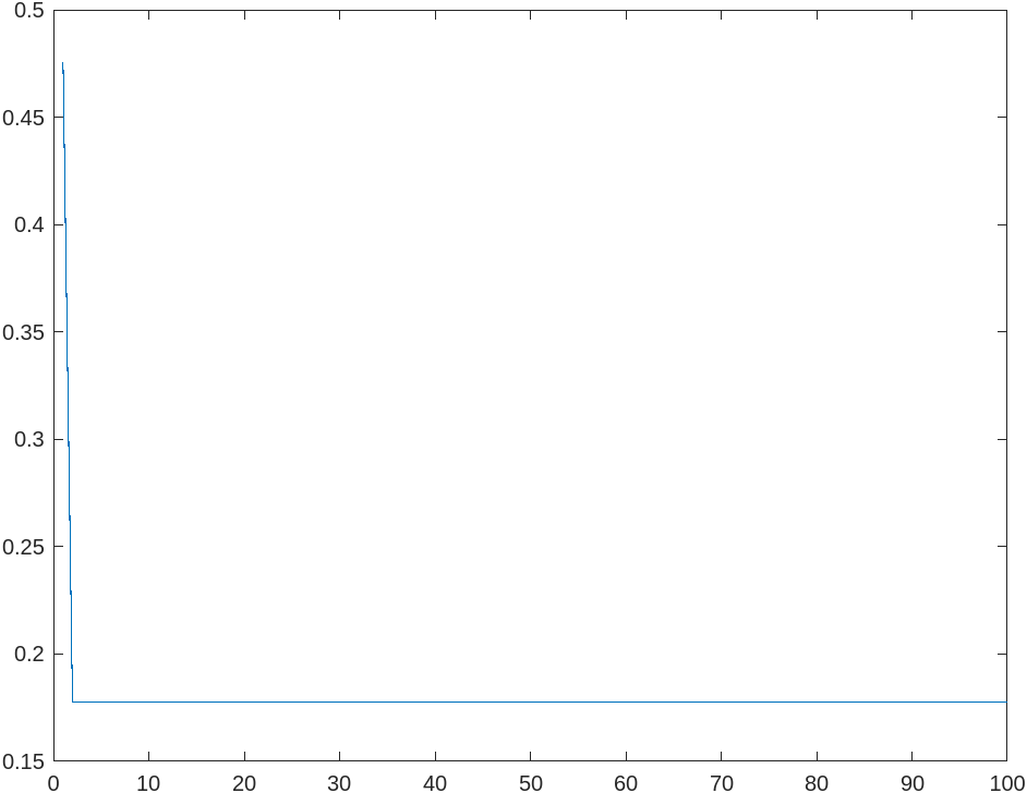
Result

it converges in 3 iterations.

ans =

    0.1778

Analysis

In the code, I use a epoch of $100$, batch size of $100$, convergence error of $10^{-5}$, and a neural network of structure $2\times 3\times 3\times 1$.

Turns out that it takes 3 iterations to converge to a root mean squared error of approximately 0.1778. As we can see here, the steepest gradiant method converges much faster than the fixed step size gradiant method.

Conjugate Gradiant Descent

function conjugate_GD()
    function[mse] = meanSquaredError(y, y_pred)
        diff = (y - y_pred).^2;
        mse = mean(diff, "all");
    end
nTrials = 100;
conjugate_step_size = 1; % start point for minimizing
epsilon = 1e-5; % minmal convergence error
[xData,yData]=getData(100,2,2338580531);
[network]=createNetwork(2,[3,3,1]);
[Weight]=getNNWeight(network);
Weight=randn(size(Weight));
RMS=NaN(nTrials,1);
[network]=setNNWeight(network,Weight);
prev_yVal = 1;
convergence = -1;
runOnce = 1;
[yVal,yintVal]=networkFProp(xData,network);
[yGrad,~]=networkBProp(network,yintVal);
g = NaN(1,25);
for i=1:size(Weight,1)
    g(i) = -2 .* dot(squeeze(yData-yVal), squeeze(yGrad(:, i, :)));
end
d = -1 .* g;
RMS(1)=meanSquaredError(yData, yVal);
for iTrial=2:nTrials
    fun = @(a) meanSquaredError(yData, networkFProp(xData, setNNWeight(network, Weight + a .* d)));
    conjugate_step_size = fminsearch(fun, conjugate_step_size);
    % update weight
    Weight = Weight + conjugate_step_size .* d;
    [network]=setNNWeight(network, Weight);
    % evaluate gradient for the next iteration
    [yVal,yintVal]=networkFProp(xData,network);
    [yGrad,~]=networkBProp(network,yintVal);
    next_g = NaN(1, 25);
    for i=1:size(Weight,1)
        next_g(i) = -2 .* dot(squeeze(yData-yVal), squeeze(yGrad(:, i, :)));
    end
    % calculate beta using the Fletcher–Reeves method
    beta = dot(transpose(next_g), next_g) ./ dot(transpose(g), g);
    d = -1 .* next_g + beta .* d;
    RMS(iTrial)=meanSquaredError(yData, yVal);
    g = next_g;
    if (all(abs(yVal - prev_yVal) < epsilon) && runOnce == 1)
        convergence = iTrial;
        runOnce = 0;
    end
    prev_yVal = yVal;
end
disp(['it converges in ' num2str(convergence) ' iterations.']);
figure;
plot(RMS);
min(RMS)
return
end

Result

it converges in 3 iterations.

ans =

    0.1778

Analysis

In the code, I use a epoch of $100$, batch size of $100$, convergence error of $10^{-5}$, and a neural network of structure $2\times 3\times 3\times 1$.

Turns out that it takes 3 iterations to converge to a root mean squared error of approximately 0.1778. As we can see here, the conjugate gradiant method performs about the same as does the steepest descent method.

Topic of Exploration

I will choose to explore the topic of:

Convergence of the algorithm for different selection of step-sizes for fixed step-size method.

Result

I will choose four different fix step sizes to explore: $1,\: 0.1,\: 0.01,\: 0.001$ with an epoch of $5000$. $\epsilon$ means the minimum error between trials for the algorithm to be considered converged.

Step Size	$\epsilon$	Trials to Converge
1	0.0001	129
0.1	0.0001	268
0.01	0.0001	702
0.001	0.0001	3042

Analysis

We can see here, as we decrease the step size by $10$, trials to converge increase by approximately $2$. It makes sense that when we take smaller steps, the iteration it takes to reach the goal will be greater.